Home / Blog / Distribution of Workforce: Where Workers Really Are
Distribution of Workforce: Where Workers Really Are
ProfessionLens, 2026-11-15
The world's workforce stopped being mostly agricultural within a single generation. Agriculture supplied 44% of global employment in 1991 and 27% by 2019, while services climbed from 34% to roughly half of all jobs, according to the International Labour Organization's sector employment analysis. That shift is real and well documented. It also hides a harder problem.
The same region, sector or employer can be described as three different sizes depending on which workforce a report counts. A licence file, a payroll survey and a count of people delivering a service are three different populations with three different totals. Analysts mix them constantly, and the mix-up survives because each figure is individually accurate.
What follows is a working guide to those counts: where workers sit by sector, how geography and occupation reshape the mix, how employer size changes the titles that exist, and the checks to run before you quote any number in a meeting.
Table of Contents
- Where Workers Sit in the Global Sector Shift
- How Geography Changes the Mix Across Rural and Urban Places
- How Profession Changes the Picture
- Licensed Is Not the Same as Working
- Why National Averages Hide Local Gaps
- Employer Size and Title Mix
- How to Check Any Distribution Count Before You Use It
- Choose the Right Population Before You Cite a Count
Where Workers Sit in the Global Sector Shift
Three different workforces can sit under one sector label: people licensed to do the work, people employed in it and people actively practicing. Distribution of workforce means the share of one clearly defined population assigned to each sector, place or employer. A licence register, a payroll survey and a count of active practitioners can each be accurate while producing a different total, so the denominator matters as much as the share.
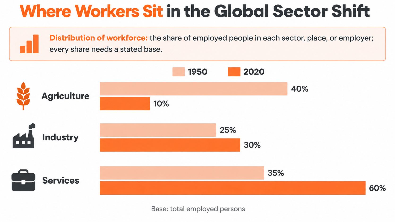
Once the base is fixed as employed people, the broad global pattern is clear:
| Sector | Direction across the shift | Reading |
|---|---|---|
| Agriculture | Fell sharply | Released a large share of labour |
| Industry | Held broadly steady | Absorbed much less of that labour than services |
| Services | Rose sharply | Became the main destination for workers leaving agriculture |
The mechanism behind the numbers
Economists call the move structural transformation. As incomes rise, households spend a smaller share of their budgets on food and more on transport, health, education, finance and technology. Labour follows that demand.
The shape of the move matters as much as its direction. Industry stayed broadly stable while services absorbed most of what agriculture released. At the global level, the main corridor out of farm work ran through services, so anyone projecting labour supply has to ask which service occupations can absorb workers and which require credentials they do not yet hold.
That last distinction is where the three populations diverge. A person can hold a licence without being employed, be employed in a sector without practicing its central occupation, or practice work that a licence register does not capture. A sector share built on employment answers where people work. It does not answer who is qualified, active or delivering the service.
Why a global average is a poor comparison
A global average works like sea level: useful for measuring movement, poor for describing any one shoreline. Each economy has a different sector mix, and the combined figure reflects both changes inside economies and each economy's weight in total employment. A large economy can move the world average even when smaller economies barely change.
Rule of thumb: a sector share is only comparable with another share built on the same sector list, the same year and the same population.
Three checks catch most errors. First, ask which classification produced the figure, because one sector list can fold retail trade and transport into services while another separates them. Second, ask whether the denominator covers all employed people, wage employees, licence holders or active practitioners. Third, distinguish a share from a headcount: a share can rise while the absolute number of jobs falls if the rest of employment shrinks faster.
Those checks also change how a services-heavy distribution should be read. A high services share can signal that work is deliverable across borders, but it says nothing by itself about skills, availability or wages. Employers using Hire talent from Latin America to build a roster therefore get more value from that share as a supply signal than as a cost estimate.
How Geography Changes the Mix Across Rural and Urban Places
Continental averages hide a spread that changes what any single share means. Africa's agricultural share of employment runs roughly double the global average, while Asia and the Pacific sits a few points above it, so a region's figure is best read against other regions rather than against the world number.
| Region or measure | Agriculture share of employment | Reading |
|---|---|---|
| Africa | Roughly double the global average | A workforce still centred on the land |
| Asia and Pacific | A few points above the global average | Large rural populations pull the share up |
| Global average | Benchmark only | Describes no single region well |
Most of the world's farm workers are not on anyone's payroll. A large share of agricultural employment is own-account and family work, so a count built on employer records or payroll systems captures only a minority of the workforce. The same land can show a large farm workforce in a household survey and a small one in employer data, and both figures can be technically accurate at the same time. The workforce didn't change. The population being counted did.
Where farm workers actually sit
Around 89% of the world's agricultural employment is based in rural areas, leaving approximately 11% in urban areas, according to the World Bank's employment-by-sector series. That series runs from 1960 to 2023 and covers 217 economies, which makes it the practical starting point for trend lines.
The rural concentration explains why farm workforces differ from urban service and industrial ones on nearly every dimension that matters: employment arrangements, productivity, social-protection coverage and measurement difficulty. A self-employed smallholder and an office employee both count as employed. Almost nothing else about their working lives lines up, which is why the survey instrument, not just the place, shapes the number you get.
Before comparing two places, ask which population produced each figure: everyone working, everyone on a payroll, or everyone licensed to work. Each describes a different workforce.
That question settles most regional disputes before they start. If one figure covers all employed people and the other covers wage employees, the gap between them may be entirely a definitional artefact rather than evidence that one region outperforms another.
How Profession Changes the Picture
Place is only half the story. Workers cluster by occupation too, and the profession mix changes how a city, state or employer looks before any other trait shows. In May 2025, office and administrative support occupations accounted for 11.4% of total U.S. employment, the largest of any major occupational group, according to the U.S. Bureau of Labor Statistics.
Think of a profession count as a menu with fixed portions. Every restaurant serves the same dishes, but the share of the plate given to each one varies. Comparing the pasta portion at two restaurants is meaningful. Comparing pasta at one against the entire menu at the other is not.
The comparison that works and the one that doesn't
Compare one occupation with itself across places. A state's registered nurses per capita against another state's registered nurses per capita is a fair test, provided both figures use the same occupation definition and the same denominator.
Comparing one occupation against the whole economy is a different exercise, and it answers a different question. A region can look under-supplied in engineering because it's unusually office-heavy, not because it lacks engineers.
Take a state where office and administrative support makes up 14% of jobs against the national 11.4%. That state is more administrative than the country as a whole. Any health or engineering comparison drawn there needs that context attached, or the reader will conclude the state is short of engineers when it is long on clerks.
Two checks before you benchmark a profession
Confirm the occupation definition matches. "Office and administrative support" bundles dozens of job titles, and a narrower local definition will produce a smaller share without any real-world change.
Confirm the denominator is total employment in the same place. A share of the local labour force and a share of a national total look identical on a chart and mean entirely different things.
Occupation mix is also the first input to serious talent market intelligence work, and the frameworks behind Visbanking's talent market intelligence guide start from exactly this question: which roles exist here, in what proportion, before anyone asks whether the supply is enough.
Licensed Is Not the Same as Working
A licence count records credentials. An employed count records jobs. A practising count records people delivering the work. The three diverge more than most reports admit, and the gap widens wherever part-time work is common, practice crosses borders or careers outlast working life.
The U.S. Bureau of Labor Statistics reported that 22.0% of employed workers held a government-issued license in 2025, while 75.1% of workers in healthcare-practitioner and technical occupations held a certification or license. Both figures come from a survey of people in jobs. Neither counts the licence records sitting on state board files, and a physician file of that kind says nothing on its own about who sees patients, where they practise, what they specialise in or whether they work full time.
| Measure | Example value | What it covers | What it misses |
|---|---|---|---|
| Employed workers holding a government-issued license (BLS, 2025) | 22.0% | Share of employed people holding a licence | Size of the licence record stock |
| Healthcare practitioner and technical workers with a certification or license (BLS, 2025) | 75.1% | Share of that occupation group | Whether those people currently practise |
| One physician licensed in four states | 4 records, 1 person | Credentials on state board files | Employment, location, specialty or hours worked |
Five statuses that get collapsed into one
Licensed means a credential exists on a file, and it may belong to someone who retired four years ago. Active is the status a board currently treats as valid, a narrower set than every record that has yet to lapse. Employed means the person appears on a payroll or in a survey, whether or not the job uses the licence. Appointed describes a person named to a role by an insurer, health system or agency, a distinction that dominates insurance producer counts. Practising means the person is delivering the service in a location, and it is the only one of the five that answers a capacity question.
Each mechanism inflates a simple count in a different way. One physician licensed in four states appears four times in a national total. Inactive credentials stay on files because renewal is cheap and surrendering them is riskier than keeping them. Remote practice detaches the licence location from the service location entirely, so even a perfectly cleaned licence file maps poorly onto where care is delivered.
A licence count, an employed count and a practising count describe three different workforces. Name which one you're quoting before anyone compares it with anything.
Licence totals overstate active capacity most in states with large retiree populations, where long careers keep the credential stock high after working supply has thinned. Counts of licensed healthcare professionals by state make the gap visible: the same state can rank near the top on credentials per capita and far lower once only working clinicians are counted.
Why National Averages Hide Local Gaps
A country can report a healthy count of doctors and still leave one province with almost none. That pattern is the norm. Health-worker density tracks national income closely, and the regions carrying the heaviest disease burdens tend to hold the thinnest workforce shares.

Rural, remote and underserved deployment stays a persistent problem, and it does not close on its own as totals grow.
Growth does not equal access
The finding that should change how you read a headline sits in the WHO's health workforce analysis: global health-worker density rose 52%, from 44.8 per 10,000 people in 2006 to 67.9 in 2025, while the same analysis still projects a global shortfall of 11.1 million health workers by 2030, concentrated mainly in low- and lower-middle-income countries. Major regional disparities persisted throughout that rise.
The world added capacity and the gaps survived.
The implication is uncomfortable for anyone tracking workforce growth as a success metric. A rising national total can coexist with a falling rural share, because new graduates cluster where the jobs, schools and hospitals already are. Turnover distorts the picture further. A region that loses three clinicians and gains three administrators posts an unchanged headcount and a weaker service position.
The test to run on any national figure
Divide the country into its regions. Weight each one by need rather than population alone, using rurality and disease burden as the weights. Then check whether the ranking changes.
If the ranking moves, the national average was hiding the story. If it holds, you can quote the national number with confidence. The same logic applies to employers building a hiring case on regional supply, and it is the reasoning behind using talent data to decide hires rather than headcount alone.
Access-adjusted measures beat raw per-capita rankings when the question is where to deploy. A state can look well staffed on a credential count and thin on a working one, so the definition matters as much as the geography. Our work on nurse practitioners by state shows why state-level counts need a population base and a status definition before they can support that kind of decision.
Employer Size and Title Mix
Company size changes which executive titles exist, and the effect shows up first in revenue and diversity roles rather than in technology. Across the Fortune 500 and Inc 5000 lists, the chief technology officer is equally common at both ends of the mid-market. The revenue and diversity titles are not.
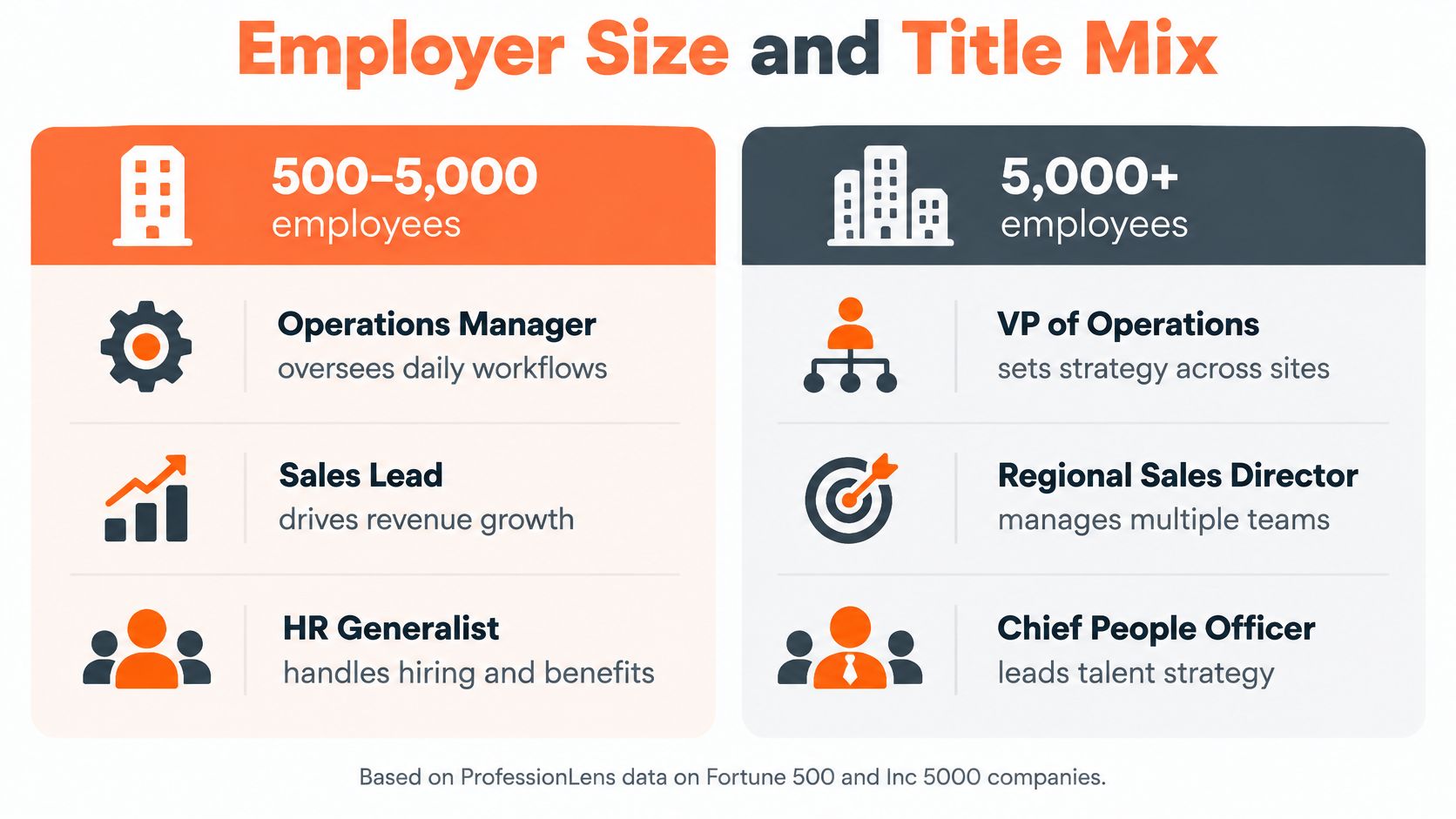
| Title | Fortune 500 | Inc 5000 | Basis |
|---|---|---|---|
| Chief technology officer | 23.1% of 117 companies | 23.1% of 208 companies | Companies with 500 to 5,000 person rows |
| Chief revenue officer | 1.7% of 117 companies | 14.4% of 208 companies | Companies with 500 to 5,000 person rows |
| Chief diversity officer | 13.5% of 483 companies | 0.0% of 4,469 companies | All companies with person rows, not limited to the 500 to 5,000 band |
The numbers reconcile once you fix the band
Compare like with like and the technology role is a tie: 23.1% of 117 Fortune 500 companies and 23.1% of 208 Inc 5000 companies within the 500 to 5,000 person band. The chief revenue officer breaks the other way, at 14.4% of Inc 5000 companies against 1.7% of Fortune 500 companies in the same band, where the Fortune 500 count sits under five.
Sector then reshapes it again inside the small-cap list. Chief revenue officers appear at 20.8% of 77 covered security companies and 16.9% of 344 covered software companies, against 3.2% of 222 consumer products companies. A revenue owner is a software and security habit more than a size effect.
The evidence gap worth stating out loud
The median Fortune 500 company in our data is seen through 10,123 person rows. The median Inc 5000 company is seen through 37. Shares for small companies therefore rest on far thinner evidence, and a single misfiled profile can move a small denominator by several points.
The denominator you can defend: every share is companies with the title divided by companies on that list with any person rows, never by the nominal 500 or 4,969.
That means 483 and 4,469 rather than 500 and 4,969, because some domains have no person rows at all. A share is published only when its base holds at least 20 rows, which is why some cells in this kind of table read as a dash rather than a percentage.
How to Check Any Distribution Count Before You Use It
Seven checks separate a figure you can cite from one that will embarrass you in a meeting. Each takes under a minute.
- Name the population. Employed, licensed, active or practicing. A licence count and an employed count can differ by a wide margin, and most reports don't say which they used.
- Check the denominator. Confirm the share divides by total employment, by the profession, or by the number of organizations with records. Dividing by a nominal list size understates every share when part of that list carries no records.
- Confirm the count date. Licence files change between releases as people renew, lapse or move out of state. A figure without a reference period can't be matched to a second figure with any confidence.
- Identify the source type. An official filing, a household survey and a self-reported profile are three different instruments. Titles on professional network profiles are self-reported, not filings, proxy statements or org charts, so they record how people present themselves.
- Check the base size. Discard any share built on fewer than 20 rows. We publish a share only when its base holds at least 20 rows, and a percentage built on 12 records is noise wearing a decimal point.
- Match the geography. State with state, county with county, employer with employer. A county figure set against a state average mostly measures the size of the county.
- Check for overlap. One professional with four state licences appears four times in a national total. De-duplicate by person before comparing capacity.
If you want to see how these checks run against published row-level data, the CSV examples from our research show the column structure behind a defensible count.
If a figure fails two or more of these checks, treat it as a rough signal. Don't build a comparison, a ranking or a budget line on it.
Choose the Right Population Before You Cite a Count
Pick the population first, then find the number. That order prevents almost every error described above, and reversing it is how analysts end up defending a figure that answers a question nobody asked.
Use licensed or active counts when the question is market size or sales capacity, because they show how many credentials and active professionals a market holds. Use employed or practicing counts when the question is service capacity or workforce planning, because those show who is available to deliver the work. A sales team sizing a territory and a hospital planning a rota need different populations from the same state.
Then fix the geographic level, national, state, county or employer, and don't mix levels inside one comparison. Record the count date alongside the figure, since files shift between releases, and match that date when you pull a second number. A figure that clears all three settings can be compared with anything built on the same definition.
We publish 17 count pages covering licensed professions nationally and in individual states, broken down by state, county or employer, with counts only and no individual names, so the population and geography you chose are the ones you get. Each research post also links the CSV of its underlying rows.
Choose your population, pull the matching count for your geography, and run the seven checks before the number reaches a slide. ProfessionLens publishes licensed-professional counts by profession, state, county and employer, plus ranked lists and research reports with the row-level CSVs behind them, so you can trace any figure back to the records that produced it. If you need to settle whether a market is short of practitioners or merely short of practicing ones, start with the count page for that profession and check the date on the file.